Decoupling stochasticity via latent variables

import matplotlib.pyplot as plt
import numpy as np
import torch; torch.set_default_dtype(torch.double)
from streaming_flow_policy.all import StreamingFlowPolicyLatent
from streaming_flow_policy.toy.plot_latent import (
    plot_probability_density_q,
    plot_probability_density_z,
    plot_probability_density_and_streamlines_q,
    plot_probability_density_and_streamlines_z,
    plot_probability_density_with_trajectories,
)

from pydrake.all import (
    CompositeTrajectory,
    PiecewisePolynomial,
    Trajectory,
)

# Set seed
np.random.seed(0)

Set hyperparameters

σ0 = 0.001
σ1 = 0.05
k = 2.5

def demonstration_traj_right() -> Trajectory:
    """
    Returns a trajectory x(t) that is 0 for 0 < t < 0.25, and a sine curve
    for 0.25 < t < 1 that starts at 0 and ends at 0.75.
    """
    piece_1 = PiecewisePolynomial.FirstOrderHold(
        breaks=[0, 0.25],
        samples=[[0, 0]],
    )
    piece_2 = PiecewisePolynomial.CubicWithContinuousSecondDerivatives(
        breaks=[0.25, 0.50, 0.75, 1.0],
        samples=[[0.00, 0.62, 0.70, 0.5]],
        sample_dot_at_start=[[0.0]],
        sample_dot_at_end=[[-0.7]],
    )
    return CompositeTrajectory([piece_1, piece_2])

def demonstration_traj_left() -> Trajectory:
    """
    Returns a trajectory x(t) that is 0 for 0 < t < 0.25, and a sine curve
    for 0.25 < t < 1 that starts at 0 and ends at 0.75.
    """
    piece_1 = PiecewisePolynomial.FirstOrderHold(
        breaks=[0, 0.25],
        samples=[[0, 0]],
    )
    piece_2 = PiecewisePolynomial.CubicWithContinuousSecondDerivatives(
        breaks=[0.25, 0.50, 0.75, 1.0],
        samples=[[0.00, -0.62, -0.70, -0.5]],
        sample_dot_at_start=[[0.0]],
        sample_dot_at_end=[[0.7]],
    )
    return CompositeTrajectory([piece_1, piece_2])

traj_right = demonstration_traj_right()
traj_left = demonstration_traj_left()

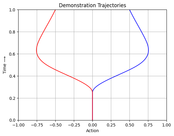
Plot demonstration trajectories

"""
Plot demonstration trajectory on x-y plane where x axis is the state in [-1, 1]
and y axis is the time in [0, 1].
"""
times = np.linspace(0, 1, 100)
plt.plot(traj_right.vector_values(times)[0], times, color='blue', alpha=0.9)
plt.plot(traj_left.vector_values(times)[0], times, color='red', alpha=0.9)
plt.xlim(-1, 1)
plt.ylim(0, 1)
plt.xlabel('Configuration')
plt.ylabel('Time ⟶')
plt.title('Demonstration Trajectories')
plt.grid(True)
plt.show()

Notation

Symbol	Space	Meaning
\(t\)	\([0, 1]\)	Time
\(q\)	\(\mathbb{C}\)	Configuration
\(z\)	\(\mathbb{C}\)	Latent variable
\(x = (q, z)\)	\(\mathbb{C}^2\)	State
\(v\)	\(\mathbb{C}^2\)	Velocity
\(o\)		Observation history
\(v_\theta(q, z, t \mid o)\)	\(\mathbb{R}^n\)	Learned flow policy
\(\xi \sim \mathcal{D}\)	\([0, 1] \rightarrow \mathbb{C}\)	Random variable for demonstration trajectories
\(\xi(t)\)	\(\mathbb{C}\)	Configuration in the demonstration at time \(t\)
\(\dot{\xi}(t)\)	\(\mathbb{C}\)	Velocity in the demonstration at time \(t\)

In this notebook, \(x \equiv q\).

Conditional flow

fp = StreamingFlowPolicyLatent(dim=1, trajectories=[traj_right], prior=[1.0], σ0=σ0, σ1=σ1, k=k)

Given \(\xi \sim \mathcal{D}\) with associated observation history \(o\), we extend the state space using a latent variable \(z \in \mathbb{C}\). We define the initial distribution at \(t = 0\) as follows.

Initial sample

\[\begin{split} \begin{align*} z_0 &\sim \mathcal{N}(0, I) \\ q_0 &\sim \mathcal{N}(\xi(0), \sigma_0^2) \end{align*} \end{split}\]

We use two hyperparameters \(\sigma_0\) and \(\sigma_1\) to represent how peaked the distribution should be at \(t = 0\) and \(t = 1\) respectively, where \(\sigma_1 \geq \sigma_0\). For convenience, define the “residual standard deviation” \(\sigma_r = \sqrt{\sigma_1^2 - \sigma_0^2 e^{-2k}}\). For an initial sample \((q_0, z_0)\), we define the flow trajectory as:

Flow trajectory

\[\begin{split} \begin{align*} q(t \mid \xi, q_0, z_0) &= \xi(t) + \left(q_0 - \xi(0)\right) e^{-kt} + (\sigma_r t)z_0 \tag{1} \\ z(t \mid \xi, q_0, z_0) &= (1 - (1 - \sigma_1)t)z_0 + t \xi(t) \tag{2} \end{align*} \end{split}\]

The flow is a diffeomorphism from \(\mathbb{C}^2\) to \(\mathbb{C}^2\) for every \(t \in [0, 1]\).

Note that \(q(0 \mid \xi, q_0, z_0) = q_0\) and \(z(0 \mid \xi, q_0, z_0) = z_0\), so the diffeomorphism is identity at \(t=0\). The marginal distribution at \(t=1\) for \(q\) and \(z\) is given by \(q(t \mid \xi) \sim \mathcal{N}(\xi(1), \sigma_1^2)\) and \(z(t \mid \xi) \sim \mathcal{N}(\xi(1), \sigma_1^2)\).

Since \((q, z)\) at time \(t\) is a linear transformation of \((q_0, z_0)\), the joint distribution of \((q, z)\) at every timestep is a Gaussian given by:

Joint distribution of (q, z) at each timestep

\[\begin{split} \begin{align*} \begin{bmatrix}q\\z\end{bmatrix} =& \underbrace{\begin{bmatrix} e^{-kt} & \sigma_r t \\ 0 & 1-(1-\sigma_1)t \end{bmatrix}}_{A}\begin{bmatrix}q_0\\z_0\end{bmatrix} + \underbrace{\begin{bmatrix}\xi(t) - \xi(0)e^{-kt}\\ t\xi{t}\end{bmatrix}}_b\\ p(q, z \mid \xi, t) =& ~\mathcal{N} \left( A \mu_0 + b \,,\, A \Sigma_0 A^T\right)\\ =& ~\mathcal{N} \left( \begin{bmatrix}\phantom{t}\xi(t)\\ t\xi(t) \end{bmatrix}, \begin{bmatrix} \Sigma_{11} & \Sigma_{12} \\ \Sigma_{12} & \Sigma_{22}\end{bmatrix}\right) \text{ where}\\ &~~\Sigma_{11} = \sigma_0^2 e^{-2kt} + \sigma_r^2 t^2 \\ &~~\Sigma_{12} = \sigma_r t \left(1 - (1-\sigma_1)t\right)\\ &~~\Sigma_{22} = \left(1 - (1-\sigma_1)t\right)^2 \end{align*} \end{split}\]

Note that \(\mu_0 = \begin{bmatrix}\xi(0)\\0 \end{bmatrix}\) and \(\Sigma_0 = \begin{bmatrix} \sigma_0^2 & 0 \\ 0 & 1\end{bmatrix}\).

At time \(t\), the velocity of the trajectory starting from \((q_0, z_0)\) is:

\[\begin{split} \begin{align*} \dot{q}(t \mid \xi, q_0, z_0) &= \dot{\xi}(t) - k\left(q_0 - \xi(0)\right) e^{-kt} + \sigma_r z_0 \tag{3} \\ \dot{z}(t \mid \xi, q_0, z_0) &= \xi(t) + t \dot{\xi}(t) - (1 - \sigma_1)z_0 \tag{4} \end{align*} \end{split}\]

The flow induces a velocity field at every \((q, z, t)\). The conditional velocity field \(v_\theta(q, z, t \mid h)\) by first inverting the flow transformation in Eq (1, 2), and plugging that into Eq. (3, 4):

• First, given \(q = q(t \mid \xi, q_0, z_0)\) and \(z = z(t \mid \xi, q_0, z_0)\), invert the flow to compute \(q_0\) and \(z_0\).

\[\begin{split} \begin{align*} z_0 &= \frac{z - t \xi(t)}{1 - (1 - \sigma_1)t} \\ q_0 &= \xi(0) + \left(q - \xi(t) - (\sigma_r t) z_0\right)e^{kt} \end{align*} \end{split}\]

• Then, plug this into Eq. (3, 4) to compute the conditional velocity field:

Conditional velocity field

\[\begin{split} \begin{align*} v_q(q, z, t \mid \xi) &= \dot{\xi}(t) - k\left( q - \xi(t) \right)+ \frac{\sigma_r \, (1 + kt)}{1 - (1 - \sigma_1)t}\left(z - t \xi(t)\right) \tag{5} \\ v_z(q, z, t \mid \xi) &= \xi(t) + t \dot{\xi}(t) - \frac{1 - \sigma_1}{1 - (1 - \sigma_1)t} \left(z - t \xi(t)\right) \tag{6} \end{align*} \end{split}\]

Plot conditional probability path of right trajectory

fig = plt.figure(figsize=(8, 4), dpi=150)

xs = torch.linspace(-1, 1, 200)
ts = torch.linspace(0, 1, 200)
ts, xs = torch.meshgrid(ts, xs, indexing='ij')  # (T, X)

gs = fig.add_gridspec(1, 2, width_ratios=[1, 1])
ax1 = fig.add_subplot(gs[0])
ax2 = fig.add_subplot(gs[1])

plot_probability_density_q(fp, ts, xs, ax1)
plot_probability_density_z(fp, ts, xs, ax2)

ax1.set_title('Configuration (q) Probability Density', size='large')
ax2.set_title('Latent Variable (z) Probability Density', size='large')

ax1.set_xlabel('Configuration (q)')
ax1.set_ylabel('Time ⟶')
ax2.set_xlabel('Latent Variable (z)')
ax2.set_ylabel('Time ⟶')

plt.tight_layout()
plt.show()

Plot conditional velocity field of right trajectory, taking expectation over other variable

fig = plt.figure(figsize=(8, 4), dpi=150)

xs = torch.linspace(-1, 1, 200)
ts = torch.linspace(0, 1, 200)
ts, xs = torch.meshgrid(ts, xs, indexing='ij')  # (T, X)

gs = fig.add_gridspec(1, 2, width_ratios=[1, 1])
ax1 = fig.add_subplot(gs[0])
ax2 = fig.add_subplot(gs[1])

plot_probability_density_and_streamlines_q(fp, ax1)
plot_probability_density_and_streamlines_z(fp, ax2)

ax1.set_title('Configuration (q) Density and Flow', size='large')
ax2.set_title('Latent Variable (z) Density and Flow', size='large')

ax1.set_xlabel('Configuration (q)')
ax1.set_ylabel('Time ⟶')
ax2.set_xlabel('Latent Variable (z)')
ax2.set_ylabel('Time ⟶')

plt.tight_layout()
plt.show()

Plot trajectories under conditional flow of right trajectory

q_starts = [0.0] * 10
z_starts_pos = np.abs(np.random.randn(5))
z_starts_neg = -np.abs(np.random.randn(5))
z_starts = sorted(np.concatenate([z_starts_neg, z_starts_pos]))
colors = ['red'] * 5 + ['red'] * 5

fig = plt.figure(figsize=(8, 4), dpi=150)

gs = fig.add_gridspec(1, 2, width_ratios=[1, 1])
ax1 = fig.add_subplot(gs[0])
ax2 = fig.add_subplot(gs[1])

plot_probability_density_with_trajectories(
    fp, ax1, ax2, q_starts, z_starts, colors, num_points_x=400,
)
plt.show()

Marginal flow

fp = StreamingFlowPolicyLatent(dim=1, trajectories=[traj_right, traj_left], prior=[0.5, 0.5], σ0=σ0, σ1=σ1, k=k)

Training

Flow matching loss:

\[ \mathcal{L}_\mathrm{FM}(\theta, \mathcal{D}) = \mathbb{E}_{\xi \sim \mathcal{D},\ t,\ x \sim x(t \mid \xi)} \big\| v_\theta(q, z, t \mid o) - v(q, z, t \mid \xi) \big\|_2^2 \]

1. Sample trajectory from dataset \(\xi \sim \mathcal{D}\).

2. Sample \(q_0 \sim \mathcal{N}(\xi(0), \sigma_0^2)\).

3. Sample \(z_0 \sim \mathcal{N}(0, I)\).

4. Sample \(t \sim \text{Uniform}([0, 1])\).

5. Compute \(q = q(t \mid \xi, q_0, z_0)\) and \(z = z(t \mid \xi, q_0, z_0)\) using Eq. (1, 2).

6. Compute conditional velocity field \(v_\theta(q, z, t \mid o)\) using Eq. (5, 6).

7. Compute L2 loss: \(\| v_\theta(q, z, t \mid o) - v(q, z, t \mid \xi) \|_2^2\).

Flow matching theorem

If \(v^*(x, t \mid o)\) is the optimal velocity field that minimizes the flow matching loss, then the marginal distributions \(\mathbb{P}^*(x \mid t, o)\) induced by \(v^*\) at every time \(t\) is the “average” of the conditional flow distributions \(\mathbb{P}(x \mid t, \xi)\) averaged over the training distribution.

\[ \mathbb{P}^*(x \mid t, o) = \mathbb{E}_{\xi} \left[ \mathbb{P}(x \mid t, \xi) \right], \ \forall x \in \mathbb{C}^2, \forall t \in [0, 1] \]

where here, \(x = (q, z)\).

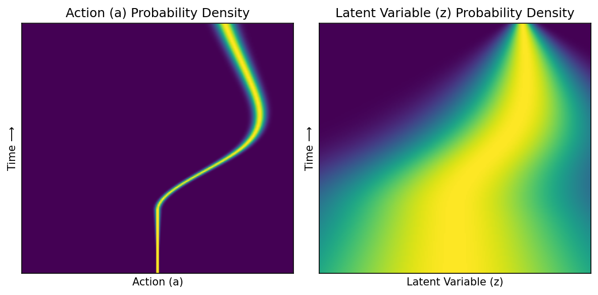
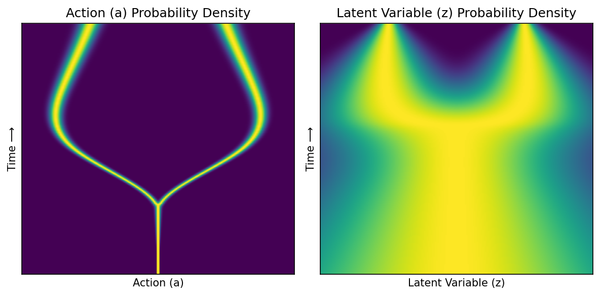
Plot marginal probability path

fig = plt.figure(figsize=(8, 4), dpi=150)

xs = torch.linspace(-1, 1, 200)  # (X,)
ts = torch.linspace(0, 1, 400)  # (T,)
ts, xs = torch.meshgrid(ts, xs, indexing='ij')  # (T, X)

gs = fig.add_gridspec(1, 2, width_ratios=[1, 1])
ax1 = fig.add_subplot(gs[0])
ax2 = fig.add_subplot(gs[1])

plot_probability_density_q(fp, ts, xs, ax1)
plot_probability_density_z(fp, ts, xs, ax2)

ax1.set_title('Configuration (q) Probability Density', size='large')
ax2.set_title('Latent Variable (z) Probability Density', size='large')

ax1.set_xlabel('Configuration (q)')
ax1.set_ylabel('Time ⟶')
ax2.set_xlabel('Latent Variable (z)')
ax2.set_ylabel('Time ⟶')

plt.tight_layout()
plt.show()

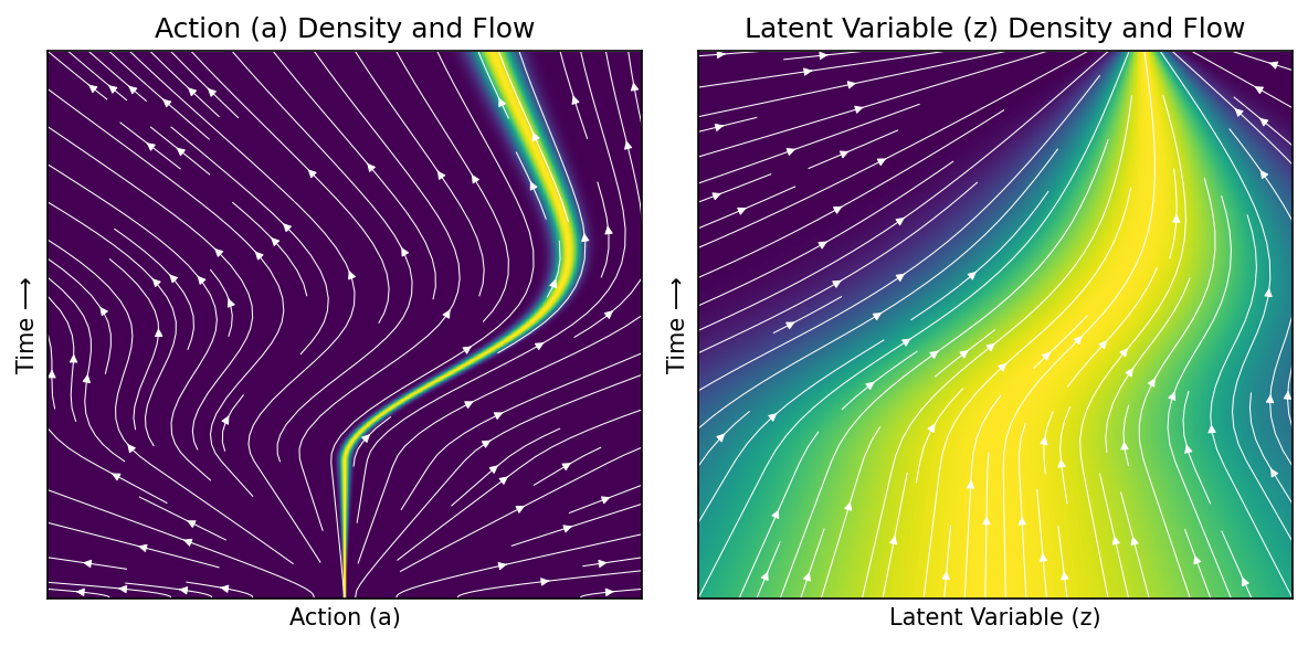
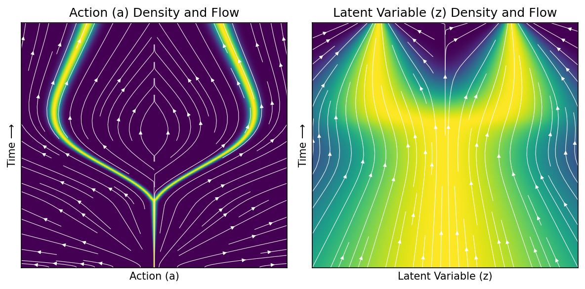
Plot marginal velocity field, taking expectation over other variable

fig = plt.figure(figsize=(8, 4), dpi=150)

xs = torch.linspace(-1, 1, 200)
ts = torch.linspace(0, 1, 200)
ts, xs = torch.meshgrid(ts, xs, indexing='ij')  # (T, X)

gs = fig.add_gridspec(1, 2, width_ratios=[1, 1])
ax1 = fig.add_subplot(gs[0])
ax2 = fig.add_subplot(gs[1])

plot_probability_density_and_streamlines_q(fp, ax1)
plot_probability_density_and_streamlines_z(fp, ax2)

ax1.set_title('Configuration (q) Density and Flow', size='large')
ax2.set_title('Latent Variable (z) Density and Flow', size='large')

ax1.set_xlabel('Configuration (q)')
ax1.set_ylabel('Time ⟶')
ax2.set_xlabel('Latent Variable (z)')
ax2.set_ylabel('Time ⟶')

plt.tight_layout()
plt.show()

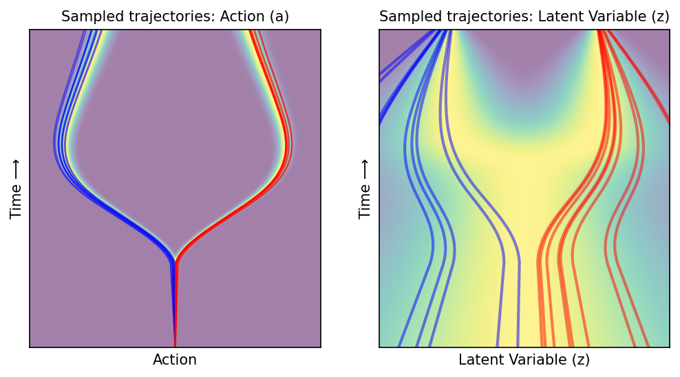
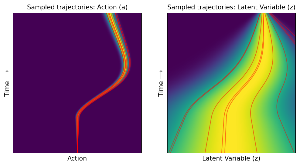
Plot trajectories under marginal flow

q_starts = [0.0] * 20
z_starts_pos = np.abs(np.random.randn(10))
z_starts_neg = -np.abs(np.random.randn(10))
z_starts = sorted(np.concatenate([z_starts_pos, z_starts_neg]))
colors = ['blue'] * 10 + ['red'] * 10

fig = plt.figure(figsize=(8, 4), dpi=150)

gs = fig.add_gridspec(1, 2, width_ratios=[1, 1])
ax1 = fig.add_subplot(gs[0])
ax2 = fig.add_subplot(gs[1])

plot_probability_density_with_trajectories(
    fp, ax1, ax2, q_starts, z_starts, colors,
    heatmap_alpha=0.5,
    linewidth_q=1, linewidth_z=2,
    num_points_x=400,
)
plt.show()