Streaming flow policy with stabilizing conditional flow

import jupyviz as jviz
import matplotlib.pyplot as plt
import numpy as np
import torch; torch.set_default_dtype(torch.double)
from streaming_flow_policy.all import StreamingFlowPolicyCSpace
from streaming_flow_policy.toy.plot_cspace import (
    plot_probability_density,
    plot_probability_density_and_vector_field,
    plot_probability_density_and_streamlines,
    plot_probability_density_with_static_trajectories,
    plot_probability_density_and_streamlines_with_animated_trajectories,
)

from pydrake.all import (
    CompositeTrajectory,
    PiecewisePolynomial,
    Trajectory,
)

# Set seed
np.random.seed(0)

Set hyperparameters

σ0 = 0.05
k = 2.5

def demonstration_traj_right() -> Trajectory:
    """
    Returns a trajectory x(t) that is 0 for 0 < t < 0.25, and a sine curve
    for 0.25 < t < 1 that starts at 0 and ends at 0.75.
    """
    piece_1 = PiecewisePolynomial.FirstOrderHold(
        breaks=[0, 0.25],
        samples=[[0, 0]],
    )
    piece_2 = PiecewisePolynomial.CubicWithContinuousSecondDerivatives(
        breaks=[0.25, 0.50, 0.75, 1.0],
        samples=[[0.00, 0.62, 0.70, 0.5]],
        sample_dot_at_start=[[0.0]],
        sample_dot_at_end=[[-0.7]],
    )
    return CompositeTrajectory([piece_1, piece_2])

def demonstration_traj_left() -> Trajectory:
    """
    Returns a trajectory x(t) that is 0 for 0 < t < 0.25, and a sine curve
    for 0.25 < t < 1 that starts at 0 and ends at 0.75.
    """
    piece_1 = PiecewisePolynomial.FirstOrderHold(
        breaks=[0, 0.25],
        samples=[[0, 0]],
    )
    piece_2 = PiecewisePolynomial.CubicWithContinuousSecondDerivatives(
        breaks=[0.25, 0.50, 0.75, 1.0],
        samples=[[0.00, -0.62, -0.70, -0.5]],
        sample_dot_at_start=[[0.0]],
        sample_dot_at_end=[[0.7]],
    )
    return CompositeTrajectory([piece_1, piece_2])

traj_right = demonstration_traj_right()
traj_left = demonstration_traj_left()

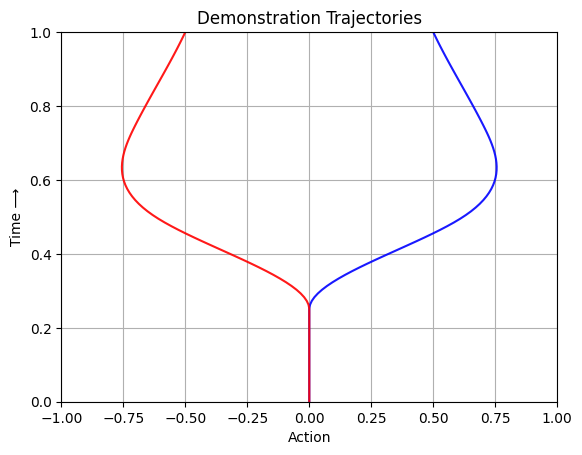
Plot demonstration trajectories

"""
Plot demonstration trajectory on x-y plane where x axis is the state in [-1, 1]
and y axis is the time in [0, 1].
"""
times = np.linspace(0, 1, 100)
plt.plot(traj_right.vector_values(times)[0], times, color='blue', alpha=0.9)
plt.plot(traj_left.vector_values(times)[0], times, color='red', alpha=0.9)
plt.xlim(-1, 1)
plt.ylim(0, 1)
plt.xlabel('Configuration')
plt.ylabel('Time ⟶')
plt.title('Demonstration Trajectories')
plt.grid(True)
plt.show()

Notation

Symbol	Space	Meaning
\(t\)	\([0, 1]\)	Time
\(q\)	\(\mathbb{C}\)	Configuration
\(x = q\)	\(\mathbb{C}\)	State (may not equal configuration in general)
\(v\)	\(\mathbb{C}\)	Velocity
\(o\)		Observation history
\(v_\theta(x, t \mid o)\)	\(\mathbb{C}\)	Learned flow policy
\(\xi \sim \mathcal{D}\)	\([0, 1] \rightarrow \mathbb{C}\)	Random variable for demonstration trajectories
\(\xi(t)\)	\(\mathbb{C}\)	Configuration in the demonstration at time \(t\)
\(\dot{\xi}(t)\)	\(\mathbb{C}\)	Velocity in the demonstration at time \(t\)

In this notebook, \(x \equiv q\).

Hyperparameters

Symbol	Space	Meaning
\(\sigma_0\)	\(\mathbb{R}_{\geq 0}\)	Initial standard deviation
\(k\)	\(\mathbb{R}_{\geq 0}\)	Stabilizing gain for the conditional flow

Conditional flow

fp = StreamingFlowPolicyCSpace(dim=1, trajectories=[traj_right], prior=[1.0], σ0=σ0, k=k)

Given \(\xi \sim \mathcal{D}\) with associated observation history \(o\), we will define a conditional flow field \(v_\theta(x, t \mid o)\) that must be learned.

First, we sample the initial configuration \(q_0\) from a Gaussian centered at the initial configuration of the demonstration trajectory:

\[ q_0 \sim \mathcal{N}(\xi(0), \sigma_0^2) \]

where \(\sigma_0\) is a small value. Then, the stabilizing velocity field is given by:

\[ \begin{align*} v(q, t \mid \xi) &= \underbrace{-k(q - \xi(t))}_{\text{Stabilization term}} ~~+~~ \hspace{-1em}\underbrace{\dot{\xi}(t)}_{\text{Path velocity}} \end{align*} \]

To solve for the actual flow, we must solve the following ordinary differential equation (ODE):

\[\begin{split} \begin{align*} \frac{\mathrm{d}q}{\mathrm{d}t} &= -k(q - \xi(t)) + \dot{\xi}(t)\\ \implies \frac{\mathrm{d}}{\mathrm{d}t} (q - \xi(t)) &= -k(q - \xi(t))\\ \implies q(t \mid \xi) &= \xi(t) ~+~ \hspace{-1em}\underbrace{\left(q_0 - \xi(0)\right) e^{-kt}}_{\text{Error decays exponentially}} \end{align*} \end{split}\]

Due to the stabilizing velocity field, the initial error \((q_0 - \xi(0))\) decays exponentially with time.

Since \(q(t \mid \xi)\) is linear in \(q_0\), the per-timestep marginal distribution of the conditional flow at any time \(t\) is a Gaussian:

\[\mathbb{P}(q \mid t, \xi) = \mathcal{N} \left( q \,\big\vert\, \xi(t)\,,\, \sigma_0^2 e^{-2kt} \right)\]

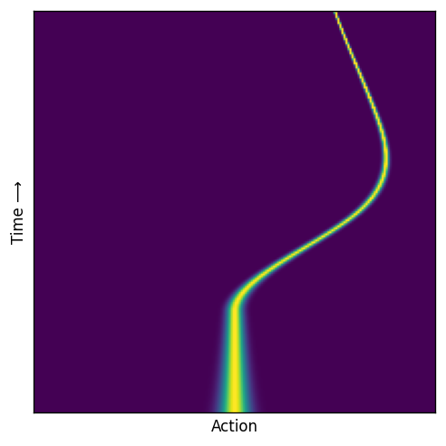
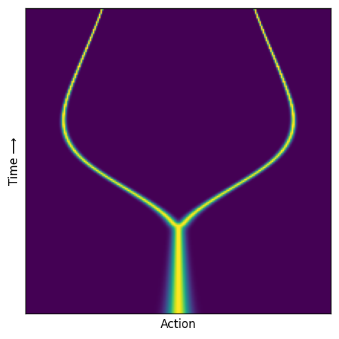
Plot conditional probability path of right trajectory

fig, ax = plt.subplots(dpi=120)
ts = torch.linspace(0, 1, 200)  # (T,)
xs = torch.linspace(-1, 1, 200)  # (X,)
ts, xs = torch.meshgrid(ts, xs, indexing='ij')  # (T, X)
plot_probability_density(fp, ts, xs, ax)
# plt.tight_layout()
plt.show()

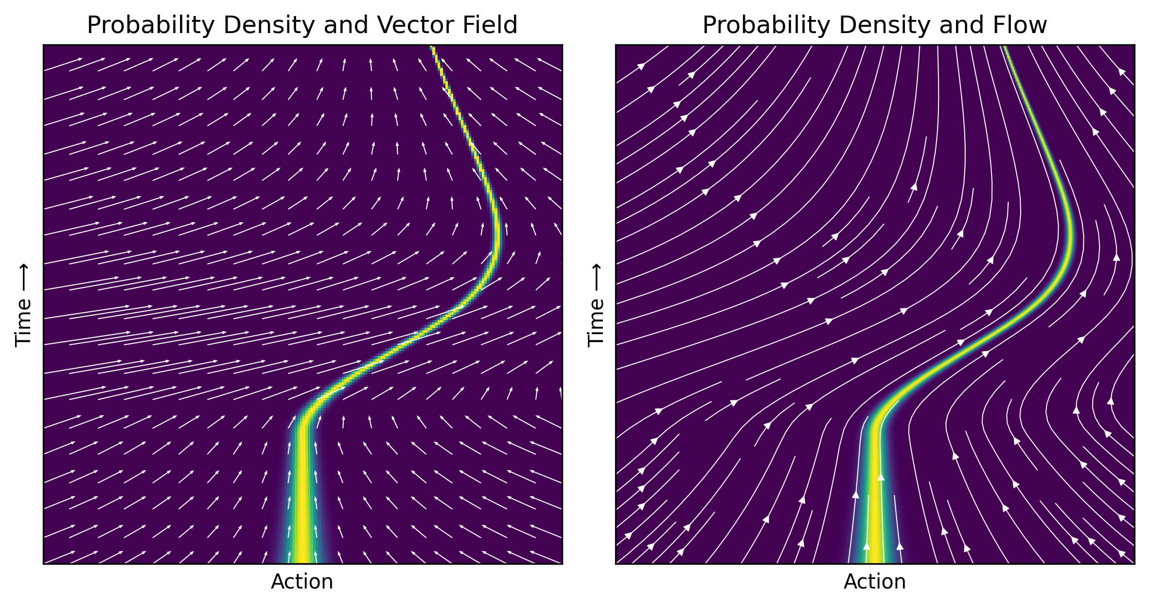
Plot conditional vector field of right trajectory

fig = plt.figure(figsize=(8, 4), dpi=300)
gs = fig.add_gridspec(1, 2, width_ratios=[1, 1])
ax1 = fig.add_subplot(gs[0])
ax2 = fig.add_subplot(gs[1])
im1 = plot_probability_density_and_vector_field(fp, ax1)
im2 = plot_probability_density_and_streamlines(fp, ax2)
plt.tight_layout()  # Uncommented to adjust spacing
plt.show()

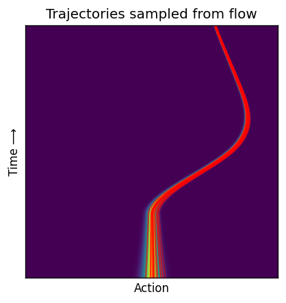
Plot trajectories under conditional flow of right trajectory

fig, ax = plt.subplots(figsize=(5, 4), dpi=120)
im = plot_probability_density_with_static_trajectories(fp, ax, [None] * 20)
plt.show()

Marginal flow

fp = StreamingFlowPolicyCSpace(dim=1, trajectories=[traj_right, traj_left], prior=[0.5, 0.5], σ0=σ0, k=k)

Training

Flow matching loss:

\[ \mathcal{L}_\mathrm{FM}(\theta, \mathcal{D}) = \mathbb{E}_{\xi \sim \mathcal{D},\ t,\ q \sim \mathcal{N}\left(\xi(t), \sigma^2\right)} \big\| v_\theta(q, t \mid o) - v(q, t \mid \xi) \big\|_2^2 \]

1. Sample trajectory from dataset \(\xi \sim \mathcal{D}\).

2. Define conditional flow \(v(q, t \mid \xi) = -k(q - \xi(t)) + \dot{\xi}(t)\).

3. Sample \(t \sim \text{Uniform}([0, 1])\).

4. Sample \(q \sim \mathcal{N} \left( q \,\big\vert\, \xi(t)\,,\, \sigma_0^2 e^{-2kt} \right)\).

5. Compute L2 loss: \(\| v_\theta(q, t \mid o) - v(q, t \mid \xi) \|_2^2\).

Flow matching theorem

If \(v^*(q, t \mid o)\) is the optimal velocity field that minimizes the flow matching loss, then the marginal distributions \(\mathbb{P}^*(q \mid t, o)\) induced by \(v^*\) at every time \(t\) is the “average” of the conditional flow distributions \(\mathbb{P}(q \mid t, \xi)\) averaged over the training distribution.

\[\mathbb{P}^*(q \mid t, o) = \mathbb{E}_{\xi} \left[ \mathbb{P}(q \mid t, \xi) \right], \ \forall q \in \mathbb{C}, \forall t \in [0, 1]\]

Plot marginal probability path

fig, ax = plt.subplots(dpi=120)
ts = torch.linspace(0, 1, 200)  # (T,)
xs = torch.linspace(-1, 1, 200)  # (X,)
ts, xs = torch.meshgrid(ts, xs, indexing='ij')  # (T, X)
plot_probability_density(fp, ts, xs, ax)
# plt.tight_layout()
plt.show()

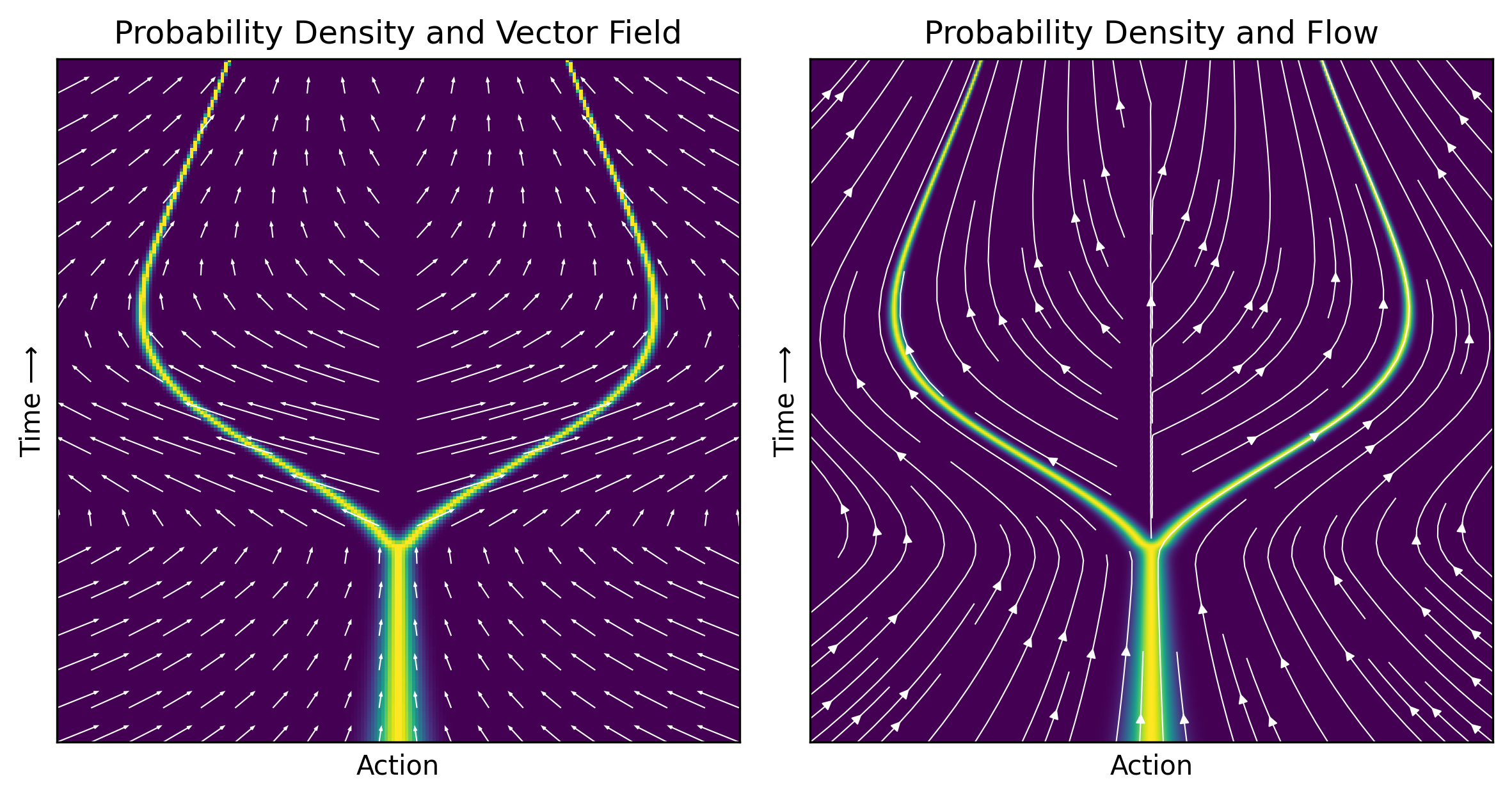
Plot marginal vector field

fig = plt.figure(figsize=(8, 4), dpi=300)
gs = fig.add_gridspec(1, 2, width_ratios=[1, 1])
ax1 = fig.add_subplot(gs[0])
ax2 = fig.add_subplot(gs[1])
im1 = plot_probability_density_and_vector_field(fp, ax1)
im2 = plot_probability_density_and_streamlines(fp, ax2)
plt.tight_layout()  # Uncommented to adjust spacing
plt.show()

Plot trajectories under marginal flow

fig, ax = plt.subplots(figsize=(5, 4), dpi=200)
frames = plot_probability_density_and_streamlines_with_animated_trajectories(fp, ax, [None] * 20, num_frames=50, circle_radius=10, dpi=200)
jviz.gif(frames, time_in_ms=3000, hold_last_frame_time_in_ms=1000).html(width=500, pixelated=False).display(); plt.close()

Pathology when starting from \(q=0\)

Let us compute the trajectory from the current configuration \(q=0\).

fig, ax = plt.subplots(figsize=(5, 4), dpi=120)
im = plot_probability_density_with_static_trajectories(fp, ax, [0], linewidth=2)
plt.tight_layout()
plt.show()

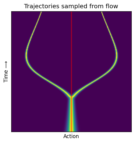
Explanation

This is due to:

1. The flow being a deterministic. Which means that for a fixed starting point (i.e. initial configuration), the trajectory is fixed.

2. In this particular example, the demonstration trajectories are symmetric. This causes the learned velocity field to be zero at \(q=0\) for all \(t \in [0, 1]\). Therefor, the sampled trajectory is pathological.

The sampled trajectory is not near the demonstration trajectories. Flow matching only guarantees that the marginal distribution of configurations is matched at each timestep. Note that the probability of exactly sampling the pathological trajectory is zero, so the flow matching guarantees are satisfied.