Streaming flow policy in the Push-T environment#
Note
This notebook is adapted from Diffusion policy’s Colab notebook with an implementation of Streaming flow policy.
# Standard imports
import collections
from dataclasses import dataclass
import gdown
import os
import numpy as np
import math
import torch
from torch import Tensor
import torch.nn as nn
from tqdm.auto import tqdm
from typing import List, Literal, Sequence, Tuple, Union

# Imports for diffusion policy
import zarr
from diffusers.schedulers.scheduling_ddpm import DDPMScheduler
from diffusers.training_utils import EMAModel
from diffusers.optimization import get_scheduler

# Imports for the Push-T environment
import gym
from gym import spaces
import pygame
import pymunk
import pymunk.pygame_util
from pymunk.space_debug_draw_options import SpaceDebugColor
from pymunk.vec2d import Vec2d
import shapely.geometry as sg
import cv2
import skimage.transform as st
import jupyviz as jviz

# always call this first
from streaming_flow_policy.all import set_random_seed
set_random_seed(0)
Push-T environment in PyMunk#
Here, we define a PyMunk-based PushTEnv environment.
This implementation is adapted from Diffusion policy, which in turn is adapted from Implicit Behavior Cloning.
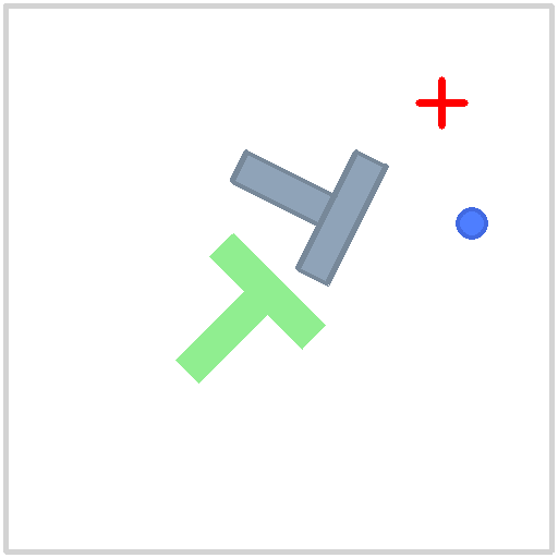
The goal is to push the gray T-block to its target position and orientation denoted in green.
PushTEnv follows the standard OpenAI Gym API (0.21.0). Here’s an illustration of the basic API calls:
# 0. create env object
env = PushTEnv()

# 1. Seed env for initial state.
# Seed 0-200 are used for the demonstration dataset.
env.seed(500)

# 2. Must reset before starting each episode.
obs, info = env.reset()

# 3. 2D positional action space [0, 512].
action = env.action_space.sample()

# 4. Stepping through environment dynamics with standard OpenAI Gym API.
obs, reward, terminated, truncated, info = env.step(action)

# 5. Render the environment.
img = env.render()  # (256, 256, 3) RGB image
jviz.img(img).html(title='Push-T render after reset').display()

# prints and explains each dimension of the observation and action vectors
with np.printoptions(precision=4, suppress=True, threshold=5):
    print("Observ: ", repr(obs))
    print("               [agent_x,  agent_y,  block_x,  block_y,    block_angle]")
    print("Action: ", repr(action) + " ⟺ [target_agent_x, target_agent_y]")

Observ:  array([314.6388, 291.4624, 301.0318, 245.9178,   0.2163])
               [agent_x,  agent_y,  block_x,  block_y,    block_angle]
Action:  array([120.8259, 101.9938]) ⟺ [target_agent_x, target_agent_y]
Demonstration dataset \(/\) dataloader#
Defines the PushTDataset (a subclass of torch.utils.data.Dataset) and helper functions.
The dataset class:
Load episodes i.e. sequences of (observation, action) tuples from a zarr storage.
Normalizes each dimension of observation and action to [-1,1].
Returns: All possible segments of length
pred_horizon. It also pads the beginning and the end of each episode with repetition, so that each timestep has a fixed number of observation length and action length. A dictionary is returned with the following signature:{ "obs": torch.Tensor of shape (`obs_horizon`, `obs_dim`), "action": torch.Tensor of shape (`pred_horizon`, `action_dim`) }
PushTDataset and dataloaders#
# Download demonstration data from Google Drive
dataset_path = "pusht_cchi_v7_replay.zarr.zip"
if not os.path.isfile(dataset_path):
    id = "1KY1InLurpMvJDRb14L9NlXT_fEsCvVUq&confirm=t"
    gdown.download(id=id, output=dataset_path, quiet=False)

# |o|o|                             observations: 2
# | |a|a|a|a|a|a|a|a|               actions executed: 8
# |p|p|p|p|p|p|p|p|p|p|p|p|p|p|p|p| actions predicted: 16

pred_horizon = 16
obs_horizon = 2
action_horizon = 8

# Create dataset from file
dataset = PushTDataset(
    dataset_path=dataset_path,
    pred_horizon=pred_horizon,
    obs_horizon=obs_horizon,
    action_horizon=action_horizon,
)
# Save training data statistics (min, max) for each dim
stats = dataset.stats

# Create dataloader
dataloader = torch.utils.data.DataLoader(
    dataset,
    batch_size=256,
    num_workers=1,
    shuffle=True,
    pin_memory=True,  # accelerate cpu-gpu transfer
    persistent_workers=True, # don't kill worker process after each epoch
)

# Visualize data in batch
batch = next(iter(dataloader))
print("batch['obs'].shape:", batch['obs'].shape)
print("batch['action'].shape", batch['action'].shape)
Downloading...
From: https://drive.google.com/uc?id=1KY1InLurpMvJDRb14L9NlXT_fEsCvVUq&confirm=t
To: /home/sancha/repos/streaming-flow-policy/notebooks/pusht/pusht_cchi_v7_replay.zarr.zip
100%|██████████| 31.1M/31.1M [00:01<00:00, 19.2MB/s]
batch['obs'].shape: torch.Size([256, 2, 5])
batch['action'].shape torch.Size([256, 16, 2])
Neural network architectures#
Defines a 1D UNet architecture ConditionalUnet1D
as the noies prediction network
Components:
SinusoidalPosEmbPositional encoding for the diffusion iteration kDownsample1dStrided convolution to reduce temporal resolutionUpsample1dTransposed convolution to increase temporal resolutionConv1dBlockConv1d –> GroupNorm –> MishConditionalResidualBlock1DTakes two inputsxandcond.
xis passed through 2Conv1dBlockstacked together with residual connection.condis applied toxwith FiLM conditioning.
Architecture changes in SFP#
We are able to re-use existing diffusion \(/\) flow policy architectures with the following changes:
Add
scaleparameter toSinusoidalPosEmb.Reason: Diffusion policy embeds integer diffusion timesteps on the order of 0 to 100, whereas flow policies use a unit interval \([0, 1]\) for time. For compatibility, we scale the unit interval by 100.
Define the two additional modules
LinearDownsample1dandLinearUpsample1d.Reason: Diffusion policy diffuses in the space of action sequences, which are processed with 1-D convolutions using
ConvUpsample1dandConvDownsample1d. However, SFP diffuses in the space of single actions. Therefore, we introduce a fully-connected upsampler\(/\)downsampler that acts on single actions.
Test neural network#
# Observation and action dimensions corresponding to the output of PushTEnv.
obs_horizon = 2
obs_dim = 5
action_dim = 2

# create network object
sfp_velocity_net = ConditionalUnet1D(
    input_dim=action_dim,
    global_cond_dim=obs_dim*obs_horizon,
    # because SFP diffuses over a single action,
    updownsample_type = 'Linear',
    # because the original model assumes timesteps of the order of [0, 100]
    # but SFP uses a time range of [0, 1]
    sin_embedding_scale = 100,
)

# Example inputs
a = torch.randn((1, 1, action_dim)) #changed SFP: action at time t
obs = torch.zeros((1, obs_horizon, obs_dim))
t = torch.zeros((1,))  # changed SFP: time t

# the velocity prediction network
# takes noisy action, diffusion iteration and observation as input
# predicts the noise added to action
with torch.no_grad():
    v = sfp_velocity_net(  # changed SFP: predicted velocity at time t
        sample=a,
        timestep=t,
        global_cond=obs.flatten(start_dim=1),
    )

# device transfer
device = torch.device('cuda')
sfp_velocity_net.to(device)

print(f"Predicted velocity shape: {v.shape}")
print(f"Predicted velocity values: {v}")
Number of parameters: 6.371482e+07
Predicted velocity shape: torch.Size([1, 1, 2])
Predicted velocity values: tensor([[[ 0.2035, -0.0741]]])
Baseline: Diffusion Policy#
Create PyTorch model for diffusion policy#
# Create network object
dp_noise_pred_net = ConditionalUnet1D(
    input_dim=action_dim,
    global_cond_dim=obs_dim*obs_horizon,
    updownsample_type = 'Conv',
    sin_embedding_scale = 1,  # original setting
)

num_diffusion_iters = 100
noise_scheduler = DDPMScheduler(
    num_train_timesteps=num_diffusion_iters,
    # the choise of beta schedule has big impact on performance
    # we found squared cosine works the best
    beta_schedule='squaredcos_cap_v2',
    # clip output to [-1,1] to improve stability
    clip_sample=True,
    # our network predicts noise (instead of denoised action)
    prediction_type='epsilon'
)

# device transfer
device = torch.device('cuda')
dp_noise_pred_net.to(device);
Number of parameters: 6.535322e+07
Diffusion policy training loop#
Takes about 4m 35s on an NVIDIA GeForce RTX 4090.
If you don’t want to wait, skip to the next cell to load pre-trained weights.
num_epochs = 100

# Exponential Moving Average
# accelerates training and improves stability
# holds a copy of the model weights
ema_dp = EMAModel(
    parameters=dp_noise_pred_net.parameters(),
    power=0.75)

# Standard ADAM optimizer
# Note that EMA parametesr are not optimized
optimizer = torch.optim.AdamW(
    params=dp_noise_pred_net.parameters(),
    lr=1e-4, weight_decay=1e-6)

# Cosine LR schedule with linear warmup
lr_scheduler = get_scheduler(
    name='cosine',
    optimizer=optimizer,
    num_warmup_steps=500,
    num_training_steps=len(dataset) * num_epochs
)

with tqdm(range(num_epochs), desc='Epoch') as tglobal:
    # epoch loop
    for epoch_idx in tglobal:
        epoch_loss = list()
        # batch loop
        with tqdm(dataloader, desc='Batch', leave=False) as tepoch:
            for nbatch in tepoch:
                # Note that the data is normalized in the dataset.
                # Device transfer
                nobs = nbatch['obs'].to(device)  # (B, To, O)
                naction = nbatch['action'].to(device)  # (B, Tp, A)
                B = nobs.shape[0]

                # Observation as FiLM conditioning
                obs_cond = nobs.flatten(start_dim=1)  # (B, To*O)

                # Sample noise to add to actions
                noise = torch.randn(naction.shape, device=device)  # (B, Tp, A)

                # sample a diffusion iteration for each data point
                timesteps = torch.randint(
                    0, noise_scheduler.config.num_train_timesteps,
                    (B,), device=device
                ).long()  # (B,)

                # Forward diffusion process: Add noise to the clean images
                # according to the noise magnitude at each diffusion iteration.
                noisy_actions = noise_scheduler.add_noise(
                    naction, noise, timesteps)  # (B, Tp, A)

                # Predict the noise residual.
                noise_pred = dp_noise_pred_net(
                    noisy_actions, timesteps, global_cond=obs_cond)

                # L2 loss
                loss = nn.functional.mse_loss(noise_pred, noise)

                # optimize
                loss.backward()
                optimizer.step()
                optimizer.zero_grad()
                # step lr scheduler every batch
                # this is different from standard pytorch behavior
                lr_scheduler.step()

                # update Exponential Moving Average of the model weights
                ema_dp.step(dp_noise_pred_net.parameters())

                # logging
                loss_cpu = loss.item()
                epoch_loss.append(loss_cpu)
                tepoch.set_postfix(loss=loss_cpu)
        tglobal.set_postfix(loss=np.mean(epoch_loss))

# Weights of the EMA model
# is used for inference
ema_noise_pred_net_dp = dp_noise_pred_net
ema_dp.copy_to(ema_noise_pred_net_dp.parameters())
Loading pretrained checkpoint (optional)#
Set load_pretrained = True to load pretrained weights.
Downloading...
From: https://drive.google.com/uc?id=1mHDr_DEZSdiGo9yecL50BBQYzR8Fjhl_&confirm=t
To: /home/sancha/repos/streaming-flow-policy/notebooks/pusht/pusht_state_100ep_dp.ckpt
100%|██████████| 261M/261M [00:11<00:00, 23.5MB/s]
Pretrained weights loaded for diffusion policy.
Diffusion policy: Inference#
Takes about 6s to roll out 200 steps on an NVIDIA GeForce RTX 4090.
# Get first observation
obs, info = env.reset()

# Keep a queue of last obs_horizon (i.e. 2) steps of observations
obs_deque = collections.deque([obs] * obs_horizon, maxlen=obs_horizon)

# Save visualization and rewards
imgs = [env.render()]
rewards = list()
done = False
step_idx = 0

max_steps = 200
with tqdm(total=max_steps, desc="Eval PushTStateEnv [Diffusion Policy]") as pbar:
    while not done:
        B = 1
        # Stack the last obs_horizon (2) number of observations.
        obs = np.stack(obs_deque)
        nobs = normalize_data(obs, stats=stats['obs'])  # normalize observation
        nobs = torch.from_numpy(nobs).to(device, dtype=torch.float32)  # device transfer

        # Infer actions: reverse diffusion process
        with torch.no_grad():
            obs_cond = nobs.unsqueeze(0).flatten(start_dim=1)  # (B, To * A)

            # Initialize action from pure Gaussian noise.
            na_traj = torch.randn(
                (1, pred_horizon, action_dim), device=device)   # (1, Tp, A)

            # Init scheduler
            noise_scheduler.set_timesteps(num_diffusion_iters)

            for k in noise_scheduler.timesteps:
                # Predict noise
                noise_pred = ema_noise_pred_net_dp(
                    sample=na_traj,
                    timestep=k,
                    global_cond=obs_cond
                )

                # Reverse diffusion (denoising) step
                na_traj = noise_scheduler.step(
                    model_output=noise_pred,
                    timestep=k,
                    sample=na_traj,
                ).prev_sample

        # Unnormalize action
        na_traj = na_traj.detach().to('cpu').numpy()  # (1, Tp, A)
        na_traj = na_traj[0]  # (Tp, A)
        a_traj = unnormalize_data(na_traj, stats=stats['action'])  # (Tp, A)

        # Only take action_horizon number of actions.
        start = obs_horizon - 1
        end = start + action_horizon
        a_traj = a_traj[start:end, :]  # (Ta, A)

        # Execute action_horizon number of steps without replanning.
        for action in a_traj:
            obs, reward, done, _, info = env.step(action)  # env step
            obs_deque.append(obs)  # collect obs
            rewards.append(reward)  # collect reward for visualization
            imgs.append(env.render())  # collect image for visualization

            # update progress bar
            step_idx += 1
            pbar.update(1)
            pbar.set_postfix(reward=reward)
            if step_idx > max_steps: done = True
            if done: break

# print out the maximum target coverage
print('Score: ', max(rewards))

# Visualize
duration_in_ms = len(imgs) * 50  # 20 FPS
jviz.gif(imgs, time_in_ms=duration_in_ms, hold_last_frame_time_in_ms=1000) \
  .html(width=256, pixelated=False, title="Diffusion policy")
Score: 0.8980183292652797

Ours: Streaming flow policy#
Generating inputs and targets for conditional flow matching loss (CFM)#
Consider an action chunk segment from the training dataset \(\mathbf{\xi} = (a_0, a_1, \dots, a_T)\).
LinearlyInterpolateTrajectory(ξ, t): Given a trajectory \(\xi: [0, 1] \to \mathcal{A}\) and time \(t \in [0, 1]\), this function linearly interpolates the trajectory to compute positions and velocities. It returns:ξt: linearly interpolated position \(\xi(t)\).dξdt: linearly interpolated velocity \(\dot{\xi}(t)\).
SampleCFMInputsAndTargets(ξt, dξdt, t, k, σ0): Samples inputs and targets for the conditional flow matching loss (CFM). It returns:a: The input action of the CFM, sampled as \(a \sim \mathcal{N}\left(\xi(t), \sigma_0^2\,e^{-2kt}\right)\). (Eq. 3 in the paper).v: The target velocity of the CFM, computed as \(v = \dot{\xi}(t) - k \left(a - \xi(t) \right)\). (Eq. 2 in the paper)
These will be used to compute the conditional flow matching loss (CFM), which is simply the \(L_2\)-distance between the velocity \(v_\theta(a, t \mid h)\) predicted by the neural network, and the target velocity \(v\).
def LinearlyInterpolateTrajectory(ξ, t):
    """
    Vectorized computation of positions and velocities if each trajectory
    (from a batch of trajectories) at given times for each trajectory, using
    linear interpolation.

    ξ (Tensor, dtype=float, shape=(B, T, A)): batch of action trajectories.
    t (Tensor, dtype=float, shape=(B,)): batch of times in [0, 1].

    Returns:
        ξt   (Tensor, shape=(B, A)): positions at time t
        dξdt (Tensor, shape=(B, A)): velocities at time t
    """
    B, T, A = ξ.shape

    # Compute the lower and upper limits of the bins that the time-points lie in.
    scaled_t = t * (T - 1)  # (B,) lies in [0, T-1]
    l = scaled_t.floor().long().clamp(0, T - 2)  # (B,) lower bin limits
    u = (l + 1).clamp(0, T - 1)  # (B,) upper bin limits
    λ = scaled_t - l.float()  # fractional part, lies in [0, 1]

    # Query the values of the upper and lower bin limits.
    batch_idx = torch.arange(B, device=ξ.device)  # (B,)
    ξl = ξ[batch_idx, l, :]  # (B, A)
    ξu = ξ[batch_idx, u, :]  # (B, A)

    # Linearly interpolate between bin limits to get position.
    λ = λ.unsqueeze(-1)  # (B, 1)
    ξt = ξl + λ * (ξu - ξl)  # (B, A)

    # Compute velocity as first-order hold.
    # Note that the time interval between two bins is Δt = 1 / (T-1).
    dξdt = (ξu - ξl) * (T - 1)  # (B, A)

    return ξt, dξdt  # (B, A) and (B, A)

def SampleCFMInputsAndTargets(ξt, dξdt, t, k, σ0):
    """
    Sample inputs and targets for the conditional flow matching loss (CFM)
    given positions and velocities at time t.

    This functions performs the following sampling (Eq. 2 and 3 of the paper):
        a ~ N(ξ(t), σ₀² exp(-2kt))  # (Eq. 3 in the paper)
        v = -k (a - ξ(t)) + dξdt(t)  # (Eq. 2 in the paper)

    Args:
        ξt (Tensor, shape=(B, A)): positions at time t.
        dξdt (Tensor, shape=(B, A)): velocities at time t.
        t (Tensor, shape=(B,)): times in [0, 1].
        k (float): Stabilizing gains of the conditional flow.
        σ0 (float): initial standard deviation of the noise added to the action.

    Returns:
        a (Tensor, shape=(B, A)): noised actions at time t
        v (Tensor, shape=(B, A)): noised action velocity targets at time t
    """
    # error = σ0 * torch.exp(-k*t).unsqueeze(1) * torch.randn_like(xt)
    t = t.unsqueeze(-1)  # (B, 1)
    sampled_error = σ0 * torch.exp(-k * t) * torch.randn_like(ξt)  # (B, A)
    a = ξt + sampled_error  # (B, A) ⟸ Eq. 3 in the paper
    v = -k * sampled_error + dξdt  # (B, A) ⟸ Eq. 2 in the paper

    return a, v  # (B, A) and (B, A)
Streaming flow policy training loop#
Takes about 3min 3s on an NVIDIA GeForce RTX 4090, which is about 33% faster than diffusion policy training (see “Diffusion policy training loop” above)
If you don’t want to wait, skip to the next cell to load pre-trained weights.
σ0 = 0.4
k = 10
num_epochs = 100

# Exponential Moving Average
# accelerates training and improves stability
# holds a copy of the model weights
ema = EMAModel(
    parameters=sfp_velocity_net.parameters(),
    power=0.75)

# Standard ADAM optimizer
# Note that EMA parametesr are not optimized
optimizer = torch.optim.AdamW(
    params=sfp_velocity_net.parameters(),
    lr=1e-4, weight_decay=1e-6)

# Cosine LR schedule with linear warmup
lr_scheduler = get_scheduler(
    name='cosine',
    optimizer=optimizer,
    num_warmup_steps=500,
    num_training_steps=len(dataloader) * num_epochs
)

with tqdm(range(num_epochs), desc='Epoch') as tglobal:
    # epoch loop
    for epoch_idx in tglobal:
        epoch_loss = list()
        # batch loop
        with tqdm(dataloader, desc='Batch', leave=False) as tepoch:
            for nbatch in tepoch:
                # Device transfer
                # Note that data is already normalized in the dataset.
                nobs = nbatch['obs'].to(device)  # (B, To, O)
                naction = nbatch['action'].to(device)  # (B, Tp, A)

                # SFP integrates actions starting from the current timestep.
                # But sequences extracted from the PushTDataset include actions
                # corresponding to the previous timesteps as well (Tp includes
                # To - 1 previous actions). The next line removes those.
                ξ = naction[:, obs_horizon-1:, :]  # (B, Tp - To + 1, A)

                # Sample t uniformly from [0, 1].
                t = torch.rand(ξ.shape[0]).float().to(device)  # (B,)

                ξt, dξdt = LinearlyInterpolateTrajectory(ξ, t)  # (B, A) and (B, A)
                a, v = SampleCFMInputsAndTargets(ξt, dξdt, t, k, σ0)  # (B, A) and (B, A)
                a, v = a.unsqueeze(1), v.unsqueeze(1)  # (B, 1, A) and (B, 1, A)

                # Conditional flow matching (CFM) loss: Mean-squared error
                # between predicted velocity and target velocity
                v̂t = sfp_velocity_net(
                    sample=a,
                    timestep=t,
                    global_cond=nobs.flatten(start_dim=1),
                )  # (B, 1, A)
                loss = nn.functional.mse_loss(v, v̂t)  # (,) L2 loss

                # optimize
                loss.backward()
                optimizer.step()
                optimizer.zero_grad()
                # step lr scheduler every batch
                # this is different from standard pytorch behavior
                lr_scheduler.step()

                # update Exponential Moving Average of the model weights
                ema.step(sfp_velocity_net.parameters())

                # logging
                loss_cpu = loss.item()
                epoch_loss.append(loss_cpu)
                tepoch.set_postfix(loss=loss_cpu)
        tglobal.set_postfix(loss=np.mean(epoch_loss))

# Weights of the EMA model
# is used for inference
ema_spf_velocity_net = sfp_velocity_net
ema.copy_to(ema_spf_velocity_net.parameters())
Loading pretrained checkpoint (optional)#
Set load_pretrained = True to load pretrained weights.
Skipped pretrained weight loading for SFP.
Streaming flow policy: Inference#
The rollout for 200 steps takes about 1.2s on an NVIDIA GeForce RTX4090, which is 5x times faster than Diffusion Policy which needs about 6s. (see the Diffusion Policy inference section above)
# Get first observation
obs, info = env.reset()

# Keep a queue of last 2 steps of observations
obs_deque = collections.deque([obs] * obs_horizon, maxlen=obs_horizon)

# Save visualization and rewards
imgs = [env.render()]
rewards = list()
done = False
step_idx = 0

# Since we are at the beginning of the episode, extract the pusher state from
# the current observation, normalize it, and use it as the "action predicted
# from the previous chunk".
a = obs[:action_dim]  # (A,)
na = normalize_data(a, stats=stats['action'])  # (A,)
na = torch.from_numpy(na).to(device, dtype=torch.float32)  # (A,)
na_from_prev_chunk = na.unsqueeze(0).unsqueeze(0)  # (1, 1, A)

max_steps = 200
with tqdm(total=max_steps, desc="Eval PushTStateEnv [Streaming Flow Policy]") as pbar:
    while not done:
        # Stack the last obs_horizon (2) number of observations
        obs = np.stack(obs_deque)  # (To, O)
        nobs = normalize_data(obs, stats=stats['obs'])  # (To, O)
        o_test = torch.from_numpy(nobs).to(device, dtype=torch.float32)  # (To, O)
        o_test = o_test.flatten().unsqueeze(0)  # (1, To * O)

        # Start integration for this action chunk from the last action
        # predicted from the previous chunk.
        # Note that "na_from_prev_chunk" is always normalized.
        na = na_from_prev_chunk  # (1, 1, A)

        # ODE integration step size
        Δt = 1.0 / (pred_horizon - obs_horizon)

        # Generate action chunk open loop i.e. the action chunk uses the same
        # observation for conditioning.
        # These actions can be streamed to execute in the environment asynchronously.
        with torch.no_grad():
            for i in range(action_horizon):

                # Stream the action to the environment (asynchronous step)
                a = na.detach().to('cpu').numpy().squeeze(axis=(0, 1))  # (A,)
                a = unnormalize_data(a, stats=stats['action'])  # (A,)
                obs, reward, done, _, info = env.step(a)  # env step
                obs_deque.append(obs)  # collect obs
                rewards.append(reward)  # collect reward for visualization
                imgs.append(env.render())  # collect image for visualization

                # Update progress bar
                step_idx += 1
                pbar.update(1)
                pbar.set_postfix(reward=reward)
                if step_idx > max_steps: done = True
                if done: break

                # Euler integration step (asynchronous).
                # Compute next action in the chunk.
                t = torch.tensor(i * Δt, device=device)  # (,) current time
                nv = ema_spf_velocity_net(
                    sample=na,  # (1, 1, A)
                    timestep=t,  # (,)
                    global_cond=o_test,  # (1, To * O)
                )  # (1, 1, A)
                na = na + nv * Δt  # (1, 1, A)

        # The last action is saved for the next chunk.
        na_from_prev_chunk = na  # (1, 1, A)

# print out the maximum target coverage
print('Score: ', max(rewards))

# Visualize
duration_in_ms = len(imgs) * 50  # 20 FPS
jviz.gif(imgs, time_in_ms=duration_in_ms, hold_last_frame_time_in_ms=1000) \
  .html(width=256, pixelated=False, title="Streaming flow policy")
Score: 0.9608730642969318
